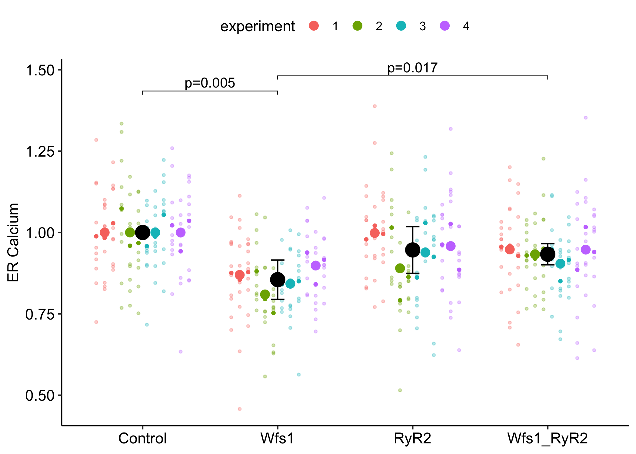
Data From Fig 2b – ER calcium depletion as a key driver for impaired ER-to-mitochondria calcium transfer and mitochondrial dysfunction in Wolfram syndrome
Fig 2b contains four replicates of an experiment, each with four treatment levels. The data were analyzed with an ANOVA model. There is nothing unusual about this. This is too bad because replicated experiments are examples of Randomized Complete Block Designs, where each experiment is a block. Analyzing blocked designs using best-practice models increases power, so the usual ANOVA model is a lost opportunity. What is highly unusual about this publication is the researchers identified the experiments in the archived data, which means I can reanalyze the data with a best practice model, either a linear mixed model or an equivalent repeated measures (RM) ANOVA. The design also contains nested technical replicates, and ignoring this is pseudorpelication, leading to increased Type I (false discoveries) error. A simulation of the Fig 2b data shows that the Type I error rate is about three times the expected rate and only with extremely low ICC does Type I error rates approach the expected rate.
nested subsampling
linear mixed model
ggplot
simulation
Author
Jeff Walker
Published
August 18, 2024
Modified
October 2, 2024
ggplot better-than-replication of Fig 2b from the article. It’s better because the plot shows the nested subsampling design…and the p-values account for this design
Fig 2b contains four replicates of an experiment, each with four treatment levels. The data were analyzed with an ANOVA model. There is nothing unusual about this. This is too bad because replicated experiments are examples of Randomized Complete Block Designs, where each experiment is a block. Analyzing blocked designs using best-practice models increases power, so the usual ANOVA model is a lost opportunity. What is highly unusual about this publication is the researchers identified the experiments in the archived data, which means I can reanalyze the data with a best practice model, either a linear mixed model or an equivalent repeated measures (RM) ANOVA.
The data in Fig 2b is actually more complex than that for a simple RCBD. In the experiment, there are four replicates of an experiment, where each experiment contains three replicate dishes for each treatment and ten measures from each dish. The researchers analyzed the data as if the sample size (n) is 10 x 3 x 4 = 120, which assumes all measurements within a treatment are independent. In fact, measures within a dish share variance, dishes within a treatment:experiment combination share variance, and dishes across treatments within an experiment share variance. The researchers’ analysis is pseudoreplicated. A simulation of the data shows that the Type I error rate, which leads to false discovery, is about three times the expected rate.
the design is actually 2 x 2 factorial but I’ll treat it as if its 4 x 0.
The experiment
Within one experimental replicate, there were three culture dishes per treatment and the researchers measured Ca++ levels in ten neurons per culture dish. The experiment was replicated four times.
From an e-mail from A. Vaarmann: “A single block corresponds to measurements from 10 neurons from one cell culture dish. Each cell culture preparation contributes at least 3 dishes to one treatment group, so 3 times 10 neurons equals 30 neurons per group. This also answers your second question. All measurements within three blocks (three blocks of 10 rows with a blank row in between blocks) correspond to one cell culture preparation i.e. n=30 per group as shown in the right panel of Fig. 1e (n = 30, 30, 30, or 29 neurons). In cases where n=60 (or more, e.g., n=90) as shown in the left panel of Fig.1e, the data from two replicate experiments are combined, with the only difference being that they are from different cell culture preparations. All other conditions are kept as similar as possible, i.e., the time between transfections and imaging, and the imaging settings.
All experiments have been repeated at least three times, i.e., with three cell culture preparations, but data from multiple cultures are combined only if the microscopy settings and the conditions between transfection and imaging are the same. That’s why the neuron n varies in different panels of the figures.”
The researchers analyzed the data as if the sample size, n, is 10 x 3 x 4 = 120, which assumes all measurements within a treatment are independent. In fact, measures within a dish share variance, dishes within a treatment:experiment combination share variance, and dishes across treatments within an experiment share variance. The researchers’ analysis is pseudoreplicated.
Setup
Fig 2b: Four experiments
Code
data_from <-"ER calcium depletion as a key driver for impaired ER-to-mitochondria calcium transfer and mitochondrial dysfunction in Wolfram syndrome"file_name <-"Source data for Figures and Table.xlsx"file_path <-here(data_folder, data_from, file_name)fig2b <-read_excel(file_path,sheet ="Fig 2B",range ="A1:F138",col_names =TRUE) |>data.table() |>melt(id.vars =c("experiment", "dish"),variable.name ="treatment_id",value.name ="er_calcium") |>na.omit()fig2b[treatment_id =="scr shRNA", treatment :="Control"]fig2b[treatment_id =="Wfs1 shRNA", treatment :="Wfs1"]fig2b[treatment_id =="RyR2 shRNA", treatment :="RyR2"]fig2b[treatment_id =="Wfs1 shRNA + RyR2 shRNA", treatment :="Wfs1_RyR2"]fig2b[, treatment :=factor(treatment,levels =c("Control", "Wfs1", "RyR2", "Wfs1_RyR2"))]fig2b[, dish_id :=ifelse(dish <10, paste0("0", dish), as.character(dish))] # for plot onlyfig2b[, dish :=paste(treatment, dish)] # dish 1 differs in each treatmentfig2b[, experiment :=as.character(experiment)] # for plot only# output as clean excel filefileout_name <-"fig2b-rcbdss-ER calcium depletion as a key driver for impaired ER-to-mitochondria calcium transfer and mitochondrial dysfunction in Wolfram syndrome.xlsx"fileout_path <-here(data_folder, data_from, fileout_name)write_xlsx(fig2b, fileout_path)
What the researchers did
The researchers fit a Linear/ANOVA model and used Sidak adjustment for the p-values. Here, I fit a linear/ANOVA model but I don’t bother adjusting since the focal p-values are really small, so the adjustment doesn’t matter. Also I don’t think the adjustment is a best strategy for most experiments like these.
Within one experimental replicate, there were three culture dishes per treatment and the researchers measured Ca++ levels in ten neurons per culture dish. The experiment was replicated four times.
The ten measures per dish are technical replicates that are not independent of each other. If the statistical model doesn’t account for this, this is pseudoreplication and inference is liberal.
The three dishes within a treatment:experiment combination are technical replicates that are not independent of each other. If the statistical model doesn’t account for this, this is pseudoreplication and inference is liberal.
The four experiments are blocks. If the statistical model doesn’t account for this, inference is conservative.
Thinking about building a best practice model
Level 1 The basic design of the experiment is a Randomized Complete Block Design (RCBD) – each experiment is a block containing all four treatment combinations.
The basic linear mixed model formula for a RCBD design is
\[y \sim treatment + (1 | experiment)\] the RM-ANOVA model for this design is
\[y \sim treatment + (treatment | experiment)\]Level 2 There are three dishes per experiment:treatment combination. I refer to the three dishes as a batch. These three dishes are subsampled (technical) replicates. If there is one measure per dish, then the design is a Randomized Complete Block Design with subsampling (RCBDS)
With three replicates within a batch, a linear mixed model can estimate treatment x experiment interactions, also known as random slopes. There are two ways of implementing this.
The interaction intercept model looks like a model with an interaction effect
The random slope and intercept model models a correlation between slope and intercept.
\[y \sim treatment + (treatment | experiment)\] The random slope/intercept model is the maximal model – it makes the fewest assumptions about the structure of the random variances and covariances.
The RM-ANOVA model for this design is
\[y \sim treatment + (treatment | experiment)\]
The RM-ANOVA model aggregates the data by analyzing the batch means.
Level 3. There are ten measures per dish. These ten measures are subsampled (technical) replicates. Since a dish is a subsampled replicate, the design has nested subsampled replicates. The design is a Randomized Complete Block Design with nested subsampling (RCBDSS).
Again, we can model this with either the interaction intercept model or the random slope and intercept model.
The RM-ANOVA model aggregates the data by analyzing the batch grand means.
Equivalencies between best practice models
If the data are balanced, the default RM-ANOVA in the afex R package is equivalent to the random slope and intercept model (this default uses a multivariate model to compute the RM-ANOVA).
In GraphPad, one might want to aggregate the data by averaging the data within a dish, then averaging these within a batch, and using RM-ANOVA. The R afex package does this automatically. This will be equivalent to the random slope and intercept model if the data are balanced.
If the data are balanced, pairwise paired t-tests on the aggregated data are equivalent to the default RM-ANOVA and to the random slope and intercept model.
These equivalencies mean that we don’t need to use LMMs if our data are balanced. The advantage of this is that LMMs can be hard to fit if there is relatively little variation in these levels relative to the variation within a dish.
A hidden problem emerges when we analyze the aggregated data with best practice models
If we plot the aggregated data, we see a second problem, which is hidden in the initial plot above but can be seen in the plot of the variation at different levels. The problem is, the data were normalized so that the mean response of the control treatment in each experiment is 1.0. The logic of this normalization is to remove the noise (non-biological) variation due to experiment. The problem is, the linear/ANOVA model of the aggregated data “thinks” the variance in the control treatment is zero and the pooled variance used for inference (the p-value), will be artificially small. The result will be slightly elevated false discoveries. While this is a minor issue, it’s easily avoided by simply not normalizing the data as the blocking variable in RM-ANOVA/LMM adjusts for this among-experiment variation. I explore
Code
fig2b_grcbd <- fig2b[, .(er_calcium =mean(er_calcium)), by = .(experiment, dish, treatment)]fig2b_rcbd <- fig2b_grcbd[, .(er_calcium =mean(er_calcium)), by = .(experiment, treatment)]
The variation of the data around each treatment mean (the residual variation) comes from four sources in the experiment:
variation among the ten cells within a dish \(\sigma^2_{cell}\)
variation among the three dish means within a batch, where a batch is a treatment:experiment combination \(\sigma^2_{dish}\)
variation among the batch means \(\sigma^2_{batch}\)
variation among the four experiments \(\sigma^2_{experiment}\)
But, inference from the linear/ANOVA model fit above and by the researchers assumes independence of the residuals, equivalent to item 1 in the list. So the linear/ANOVA model assumes zero variation in items 2 – 4 above.
A quick way to explore variation in items 2 – 4, relative to variation in item 1, is a simple plot of the residuals of the linear/ANOVA model (so there is no variation due to treatment), and ploting the batch (treatment:experiment) and dish means.
The plot shows small variation among dishes, among batches, and among experiments, relative to variation within a dish. But, how close to zero variation do we need to be to have nominal Type I error (5% if we set alpha to 0.05)?
We can measure this with a ratio of the variance at each level relative to the total random variance. These ratios are called intraclass correlations. The total random variance \(\sigma^2\) is
We can also measure the ICC at the level of the batch, dish, or experiment alone.
The problem with these data is that the variances are artificially shrunken due to the normalization described above (the data were normalized to make the control treatment mean for each experiment equal to one). So, I compute two sets of variance components: 1) the first uses all of the data, 2) the second uses only the data from the non-control groups, so the experiment component should be more similar to that had the data not been normalized.
The table below shows both computations of the three difference variance components (“Residual” is the variance among cells within a dish) used to compute the various ICCs.
Code
# (1 | experiment) - block intercept. Variance among experiments# (1 | treatment:experiment) - treatment:experiment intercept. This is mean of batch of three dishes# (1 | treatment:experiment:dish) - dish intercept. This is mean of 10 cells within a dish# Residual - this is variance among cells within a dishlmm1 <-lmer(er_calcium ~ treatment + (1| experiment) + (1| treatment:experiment) + (1| treatment:experiment:dish),data = fig2b)var_table_1 <-VarCorr(lmm1) |>as.data.frame()var_table_1$source =c("dish", "batch", "experiment", "cell")var_table_1 <- var_table_1[, c(1, 6, 4, 5)]lmm2 <-lmer(er_calcium ~ treatment + (1| experiment) + (1| treatment:experiment) + (1| treatment:experiment:dish),data = fig2b[treatment !="Control"])var_table_2 <-VarCorr(lmm2) |>as.data.frame()var_table_2$source =c("dish", "batch", "experiment", "cell")var_table_2 <- var_table_2[, c(1, 6, 4, 5)]var_table <-rbind(var_table_1, var_table_2)var_table |>kable(digits =4) |>kable_styling() |>pack_rows("All treatments", 1, 4) |>pack_rows("Non-control treatments", 5, 8)
grp
source
vcov
sdcor
All treatments
treatment:experiment:dish
dish
0.0012
0.0348
treatment:experiment
batch
0.0000
0.0000
experiment
experiment
0.0003
0.0164
Residual
cell
0.0163
0.1276
Non-control treatments
treatment:experiment:dish
dish
0.0014
0.0379
treatment:experiment
batch
0.0000
0.0000
experiment
experiment
0.0006
0.0237
Residual
cell
0.0159
0.1260
The table below are the various ICCs computed from the variance components above
The low ICC (0.113) shows that, indeed, the data in figure 2b are pretty independent. The table also shows that most (72%) of the non-residual random variance is due to dish.
How much does this small non-independence affect Type I error rate? We’ll explore this with a simulation below, but first, fit some best practice models.
Fitting best practice models
Linear mixed models
Linear mixed models have the flexibility to model all levels of variance in data like these but the solutions are not exact as in linear/ANOVA models, and they will often have a “boundary error” when variance is low at one or more levels. This happens with any of the models with the batch (treatment:experiment) intercept, which means variation among these batch means is small. The result of a model fit with a boundary layer is the collapse of this level, which will tend to have slightly inflated type I (false discovery) error. The LMM that fits without a boundary error is the simple RCBD of the completely aggregated data, which is equivalent to a paired t-test when there are only two treatment levels.
Code
# (1 | experiment) - block intercept. Variance among experiments# (1 | treatment:experiment) - treatment:experiment intercept. This is mean of batch of three dishes# (1 | treatment:experiment:dish) - dish intercept. This is mean of 10 cells within a dish# Residual - this is variance among cells within a dishlmm1 <-lmer(er_calcium ~ treatment + (1| experiment) + (1| treatment:experiment) + (1| treatment:experiment:dish), data = fig2b)# aggregate dish modellmm2 <-lmer(er_calcium ~ treatment + (1| experiment) + (1| treatment:experiment), data = fig2b_grcbd)# RCBD modellmm3 <-lmer(er_calcium ~ treatment + (1| experiment), data = fig2b_rcbd)lmm3_emm <-emmeans(lmm3, specs ="treatment")lmm3_pairs <-contrast(lmm3_emm, method ="revpairwise", adjust ="none") |>summary(infer =TRUE)gg1 <-plot_response(lmm3, lmm3_emm, lmm3_pairs[c(1,5),],palette ="pal_okabe_ito_blue")
Repeated measures ANOVA model
Repeated measures ANOVA is the punching bag of biostatistics but the multivariate-response version of RM-ANOVA is equivalent to a LMM with random slope and intercept if the nested sets of data are balanced. These data are balanced.
Code
aov1 <-aov_4(er_calcium ~ treatment + (treatment | experiment),fun_aggregate = mean,data = fig2b)aov1_emm <-emmeans(aov1, specs ="treatment")aov1_pairs <-contrast(aov1_emm, method ="revpairwise", adjust ="none") |>summary(infer =TRUE)gg2 <-plot_response(aov1, aov1_emm, aov1_pairs[c(1,5),],palette ="pal_okabe_ito_blue")# to show that the above does the aggregation # aov2 <- aov_4(er_calcium ~ treatment + (treatment | experiment),# data = fig2b_rcbd)# aov2_emm <- emmeans(aov2, specs = "treatment")# aov2_pairs <- contrast(aov2_emm, method = "revpairwise", adjust = "none") |># summary(infer = TRUE)
Pairwise paired t-tests
Pairwise paired t-tests are also equivalent to a random slope and intercept model if the nested sets are balanced. The advantage of this over a RM-ANOVA is that we can use more of the treatment:experiment combiantions if there is imbalance.
A simulation to explore false discovery when the data look pretty independent
The principal question that this simulation addresses is, how much does pseudoreplication increase type I error when ICC is low? Here I create fake data with three levels of error variance, as in Fig 2b
among cells within a dish
among replicate dishes within a treatment:experiment combination
among experimental replicates
I simulate all combinations of:
ICC = 0.05, 0.1, 0.15
Code
do_it <-FALSEset.seed(1)type_1_matrix <-data.table(NULL)if(do_it ==TRUE){ n_iter <-10000 n_cell <-10 n_dish <-3 n_exper <-4 n_treat <-4# number of treatments t_batch <- n_treat * n_exper t_dish <- n_dish * t_batch t_cell <- t_dish * n_cell beta_1 <-rep(0, n_treat) b_treat_col <-rep(beta_1, each = n_cell * n_dish * n_exper) # the fixed effects var_table_2 <-data.table(var_table_2) var_table_2[, frac_of_whole := vcov/sum(var_table_2[, vcov])] var_table_2[, frac_of_modeled := vcov/sum(var_table_2[1:3, vcov])]# unmodeled random variance is 88.8 %# dish has 72% of modeled random variance# batch has 0 % of modeled random variance# experiment has 28% of modeled random variance sigma <-1# this is the root variance lm(y ~ treatment) residual_frac_list <-c(0.9, 0.95, 0.85) # fraction of random variance that is unmodeled noise dish_frac <- .72-0.05/2 batch_frac <-0.05 exp_frac <- .28-0.05/2# ICC residual_var <- residual_frac_list * sigma^2# residual variance or variance among cells in a dish random_var <- sigma^2- residual_var # total random variance exper_var <- exp_frac * random_var # variance among experiments batch_var <- batch_frac * random_var # variance among batch of three dishes means dish_var <- dish_frac * random_var # variance among dish means icc <- (exper_var + batch_var + dish_var)/sigma^2# dish_frac + batch_frac + exp_frac # check! param_mat <-expand.grid(residual_frac = residual_frac_list) |>data.table() p1_m1 <-numeric(n_iter) p2_m1 <-numeric(n_iter) p1_m2 <-numeric(n_iter) p2_m2 <-numeric(n_iter) p1_lmm1 <-numeric(n_iter) p2_lmm1 <-numeric(n_iter) p1_aov1 <-numeric(n_iter) p2_aov1 <-numeric(n_iter)for(param_set in1:nrow(param_mat)){ residual_frac_i <- param_mat[param_set, residual_frac] # fraction of random variance that is unmodeled noise# total variance is 1 residual_var <- residual_frac_i * sigma^2# residual variance or variance among cells in a dish random_var <- sigma^2- residual_var # total random variance exper_var <- exp_frac * random_var # variance among experiments batch_var <- batch_frac * random_var # variance among batch of three dishes means dish_var <- dish_frac * random_var # variance among dish means sigma_cell <-sqrt(residual_var) # among cells within a dish - this is residual sigma_exper <-sqrt(exper_var) # among experiments sigma_batch <-sqrt(batch_var) # among batches within a treatment:experiment sigma_dish <-sqrt(dish_var) # among dishes within a treatment:experiment:batch fd <-data.table(treatment =rep(paste0("Trt", 1:n_treat), each = n_exper * n_dish * n_cell),experiment =rep(rep(paste0("exper_", 1:n_exper), each = n_dish * n_cell), 2),batch =rep(paste0("batch_", 1:t_batch), each = n_dish * n_cell),dish =rep(paste0("dish_", 1:t_dish), each = n_cell),cell =paste0("cell_", 1:t_cell),y =rep(NA, t_cell) )for(iter in1:n_iter){ b_exper <-rnorm(n_exper, mean =0, sd = sigma_exper) b_exper_col <-rep(rep(b_exper, each = n_dish * n_cell), n_treat)# length(b_exper_col) b_batch <-rnorm(t_batch, mean =0, sd = sigma_batch) b_batch_col <-rep(b_batch, each = n_dish * n_cell)# length(b_batch_col) b_dish <-rnorm(t_dish, mean =0, sd = sigma_dish) b_dish_col <-rep(b_dish, each = n_cell)# length(b_dish_col) b_cell_col <-rnorm(t_cell, mean =0, sd = sigma_cell)# length(b_cell_col)# put it all together fd[, y := b_treat_col + b_exper_col + b_batch_col + b_dish_col + b_cell_col]# lm of raw data m1 <-lm(y ~ treatment, data = fd) m1_pairs <-emmeans(m1, specs ="treatment") |>contrast(method ="revpairwise", adjust ="none") |>summary() p1_m1[iter] <- m1_pairs[1, "p.value"] p2_m1[iter] <- m1_pairs[5, "p.value"]# lm of control centered data exper_means <- fd[, .(y_bar =mean(y)), by = .(treatment, experiment)] y_bar_vec <-rep(rep(exper_means[1:4, y_bar], each = n_cell * n_dish), 4) fd[, y_c := y/y_bar_vec]# fd[, .(mean = mean(y_c),# sd = sd(y_c)), by = .(treatment, experiment)] m2 <-lm(y_c ~ treatment, data = fd) m2_pairs <-emmeans(m2, specs ="treatment") |>contrast(method ="revpairwise", adjust ="none") |>summary() p1_m2[iter] <- m2_pairs[1, "p.value"] p2_m2[iter] <- m2_pairs[5, "p.value"]# lmm models lmm1 <-lmer(y ~ treatment + (1| experiment) + (1| batch) + (1| dish), data = fd) lmm1_pairs <-emmeans(lmm1, specs ="treatment") |>contrast(method ="revpairwise", adjust ="none") |>summary() p1_lmm1[iter] <- lmm1_pairs[1, "p.value"] p2_lmm1[iter] <- lmm1_pairs[5, "p.value"]# RM-ANOVA models aov1 <-aov_4(y ~ treatment + (treatment | experiment), data = fd, fun_aggregate = mean) aov1_pairs <-emmeans(aov1, specs ="treatment") |>contrast(method ="revpairwise", adjust ="none") |>summary() p1_aov1[iter] <- aov1_pairs[1, "p.value"] p2_aov1[iter] <- aov1_pairs[5, "p.value"] } type_1_matrix <-rbind( type_1_matrix,data.table(resid_frac = residual_frac_i,"sigma_cell"= sigma_cell, # among cells within a dish - this is residual"sigma_exper"= sigma_exper, # among experiments"sigma_batch"= sigma_batch, # among batches within a treatment:experiment"sigma_dish"= sigma_dish, # among dishes within a treatment:experiment:batch"p1_m1"= p1_m1,"p2_m1"= p2_m1,"p1_m2"= p1_m2,"p2_m2"= p2_m2,"p1_lmm1"= p1_lmm1,"p2_lmm1"= p2_lmm1,# "p1_lmm2" = p1_lmm2,# "p2_lmm2" = p2_lmm2,"p1_aov1"= p1_aov1,"p2_aov1"= p2_aov1 ) ) }saveRDS(type_1_matrix, "type_1_matrix.Rds")}else{ type_1_matrix <-readRDS("type_1_matrix.Rds")}residual_frac_list <-unique(type_1_matrix$resid_frac)param_mat <-expand.grid(residual_frac = residual_frac_list)param_mat$icc <-NAparam_mat$lm1_p1 <-NAparam_mat$lm1_p2 <-NAparam_mat$lm2_p1 <-NAparam_mat$lm2_p2 <-NAparam_mat$lmm1_p1 <-NAparam_mat$lmm1_p2 <-NAparam_mat$rmaov_p1 <-NAparam_mat$rmaov_p2 <-NAfor(param_set in1:nrow(param_mat)){ residual_frac_i <- param_mat[param_set, "residual_frac"] # fraction of random variance that is unmodeled noise random_var <- type_1_matrix[resid_frac == residual_frac_i, sigma_exper][1]^2+ type_1_matrix[resid_frac == residual_frac_i, sigma_batch][1]^2+ type_1_matrix[resid_frac == residual_frac_i, sigma_dish][1]^2 total_var <- random_var + type_1_matrix[resid_frac == residual_frac_i, sigma_cell][1]^2 param_mat[param_set, "icc"] <- random_var/total_var p1_m1 <- type_1_matrix[resid_frac == residual_frac_i, p1_m1] p2_m1 <- type_1_matrix[resid_frac == residual_frac_i, p2_m1] p1_m2 <- type_1_matrix[resid_frac == residual_frac_i, p1_m2] p2_m2 <- type_1_matrix[resid_frac == residual_frac_i, p2_m2] p1_lmm1 <- type_1_matrix[resid_frac == residual_frac_i, p1_lmm1] p2_lmm1 <- type_1_matrix[resid_frac == residual_frac_i, p2_lmm1] p1_aov1 <- type_1_matrix[resid_frac == residual_frac_i, p1_aov1] p2_aov1 <- type_1_matrix[resid_frac == residual_frac_i, p2_aov1] n_iter <-length(p1_m1) param_mat[param_set, "lm1_p1"] <-sum(p1_m1 <0.05)/n_iter param_mat[param_set, "lm1_p2"] <-sum(p2_m1 <0.05)/n_iter param_mat[param_set, "lmm1_p1"] <-sum(p1_lmm1 <0.05)/n_iter param_mat[param_set, "lmm1_p2"] <-sum(p2_lmm1 <0.05)/n_iter param_mat[param_set, "lm2_p1"] <-sum(p1_m2 <0.05)/n_iter param_mat[param_set, "lm2_p2"] <-sum(p2_m2 <0.05)/n_iter param_mat[param_set, "rmaov_p1"] <-sum(p1_aov1 <0.05)/n_iter param_mat[param_set, "rmaov_p2"] <-sum(p2_aov1 <0.05)/n_iter}param_mat |>kable(digits =c(2,2,3,3,3,3,3,3,3,3)) |>kable_styling()
Even though the dependence due to shared variance seems small given the figure of this variance above, the Type I error rate is 14.4% - 14.9%, or almost 3X the expected rate of 5%. This is an unacceptable inflation of type I error that will lead to frequent false discovery. By contrast, the RM-ANOVA model has exceptional control of Type I error rate. And, the naive LMM is overly conservative.
Key:
lm1: Linear/ANOVA model of all data, ignoring nesting. The data are not normalized by the mean of the control.
lm2: Linear/ANOVA model of the control-normalized data, ignoring nesting. This is what the researchers did
lmm1: Linear mixed model with intercepts for experiment, batch (= treatment:experiment), and dish. A naive model that simply accepts results regardless of boundary errors.
aov1: multivariate Repeated Measures ANOVA
Exploring other figure panels
Fig 1c
Code
data_from <-"ER calcium depletion as a key driver for impaired ER-to-mitochondria calcium transfer and mitochondrial dysfunction in Wolfram syndrome"file_name <-"Source data for Figures and Table.xlsx"file_path <-here(data_folder, data_from, file_name)fig1c <-read_excel(file_path,sheet ="Fig 1C",range ="A1:D56",col_names =TRUE) |>data.table() |>melt(id.vars =c("dish"),variable.name ="treatment",value.name ="er_calcium") |>na.omit()fig1c[, dish_id :=as.character(dish)]fig1c[, dish :=paste(treatment, dish)]# output as clean excel filefileout_name <-"fig1c-ER calcium depletion as a key driver for impaired ER-to-mitochondria calcium transfer and mitochondrial dysfunction in Wolfram syndrome.xlsx"fileout_path <-here(data_folder, data_from, fileout_name)write_xlsx(fig1c, fileout_path)
data_from <-"ER calcium depletion as a key driver for impaired ER-to-mitochondria calcium transfer and mitochondrial dysfunction in Wolfram syndrome"file_name <-"Source data for Figures and Table.xlsx"file_path <-here(data_folder, data_from, file_name)fig1e_left <-read_excel(file_path,sheet ="Fig 1E",range ="A1:F67",col_names =TRUE) |>data.table() |>melt(id.vars =c("experiment", "dish"),variable.name ="treatment",value.name ="er_calcium") |>na.omit()fig1e_left[, dish_id :=as.character(dish)] # for plot onlyfig1e_left[, dish :=paste(treatment, dish)] # dish 1 differs in each treatment# output as clean excel file# fileout_name <- "fig1c-ER calcium depletion as a key driver for impaired ER-to-mitochondria calcium transfer and mitochondrial dysfunction in Wolfram syndrome.xlsx"# fileout_path <- here(data_folder, data_from, fileout_name)# write_xlsx(fig1c, fileout_path)
data_from <-"ER calcium depletion as a key driver for impaired ER-to-mitochondria calcium transfer and mitochondrial dysfunction in Wolfram syndrome"file_name <-"Source data for Figures and Table.xlsx"file_path <-here(data_folder, data_from, file_name)fig1e_right <-read_excel(file_path,sheet ="Fig 1E",range ="F1:J34",col_names =TRUE) |>data.table() |>melt(id.vars =c("dish"),variable.name ="treatment",value.name ="er_calcium") |>na.omit()fig1e_right[, dish_id :=as.character(dish)] # for plot onlyfig1e_right[, dish :=paste(treatment, dish)] # dish 1 differs in each treatment# output as clean excel file# fileout_name <- "fig1c-ER calcium depletion as a key driver for impaired ER-to-mitochondria calcium transfer and mitochondrial dysfunction in Wolfram syndrome.xlsx"# fileout_path <- here(data_folder, data_from, fileout_name)# write_xlsx(fig1c, fileout_path)
data_from <-"ER calcium depletion as a key driver for impaired ER-to-mitochondria calcium transfer and mitochondrial dysfunction in Wolfram syndrome"file_name <-"Source data for Figures and Table.xlsx"file_path <-here(data_folder, data_from, file_name)fig8c_wide <-read_excel(file_path,sheet ="Fig 8C",range ="G1:L164",col_names =TRUE) |>data.table() |>na.omit()fig8c <-melt(fig8c_wide,id.vars =c("experiment", "dish"),variable.name ="treatment",value.name ="number_with_mitochondria")fig8c[, dish_id :=ifelse(dish <10, paste0("0", dish), as.character(dish))] # for plot onlyfig8c[, dish :=paste(treatment, dish)] # dish 1 differs in each treatmentfig8c[, experiment :=as.character(experiment)] # for plot only# output as clean excel filefileout_name <-"fig8c-ER calcium depletion as a key driver for impaired ER-to-mitochondria calcium transfer and mitochondrial dysfunction in Wolfram syndrome.xlsx"fileout_path <-here(data_folder, data_from, fileout_name)write_xlsx(fig8c, fileout_path)